Making section plots with oce and `imagep()`

2016-04-25 in OCE • R
section ctd plots imagep colormap ctd
3 min read

section objects in the oce package are a convenient way of storing a series of CTD casts together – indeed, the object name derives from the common name for such a series of casts collected from a ship during a single campaign.

In it’s heart, a section object is really just a collection of ctd objects, with some other metadata. The CTD stations themselves are stored as a list of ctd objects in the @data slot, like:

library(oce)
data(section)
str(section@data$station, 1)

List of 124
 $ :Formal class 'ctd' [package "oce"] with 3 slots
 $ :Formal class 'ctd' [package "oce"] with 3 slots
 $ :Formal class 'ctd' [package "oce"] with 3 slots
 $ :Formal class 'ctd' [package "oce"] with 3 slots
 $ :Formal class 'ctd' [package "oce"] with 3 slots
 $ :Formal class 'ctd' [package "oce"] with 3 slots
 $ :Formal class 'ctd' [package "oce"] with 3 slots
 $ :Formal class 'ctd' [package "oce"] with 3 slots
  [list output truncated]

Just to prove it, we can plot make a standard ctd plot of one of them, by accessing them directly with the [[ accessor syntax. Let’s plot the 100th station:

plot(section[['station']][[100]])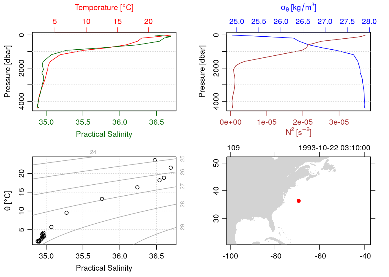

Making nice plots of the sections themselves

The main advantage of a section object is to be able to quickly make plots summarizing all the data in the section. This is accomplished using the plot method for section objects, which you can read about by doing ?"plot,section-method". For example, to make a contour plot of the temperature:

plot(section, which='temperature', xtype='distance')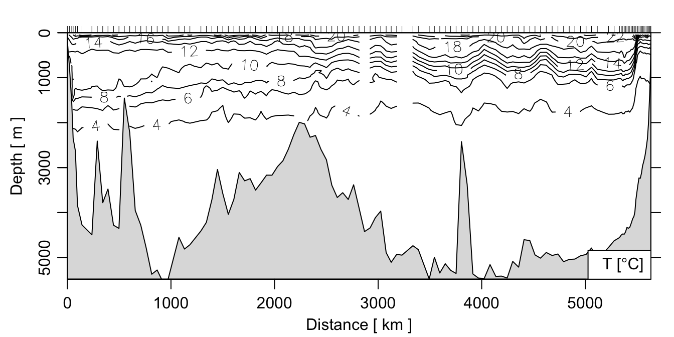

Ok, cool. But what about some colors? Use the ztype='image' argument!

plot(section, which='temperature', xtype='distance',
     ztype='image')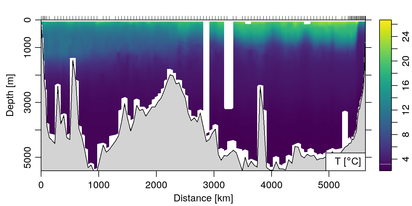

Finer control over the section plot

To get finer control over the section plot than is possible with the section plot() method, one trick I will sometimes do is extract the data I want from the section as a gridded matrix, and then plot the matrix directly using the imagep() function.

First, we “grid” the section so that all the stations comprise the same pressure levels:

s <- sectionGrid(section, p='levitus')

Now, we can loop through the station fields, extracting the data as we go.

nstation <- length(s[['station']])
p <- unique(s[['pressure']])
np <- length(p)
T <- S <- array(NA, dim=c(nstation, np))
for (i in 1:nstation) {
    T[i, ] <- s[['station']][[i]][['temperature']]
    S[i, ] <- s[['station']][[i]][['salinity']]
}

Basically, what we’re doing here is creating an empty matrix, then filling each row with the data from the section stations. We can make a quick plot with imagep():

distance <- unique(s[['distance']])
par(mfrow=c(2, 1))
imagep(distance, p, T, col=oceColorsTemperature, flipy=TRUE)
imagep(distance, p, S, col=oceColorsSalinity, flipy=TRUE)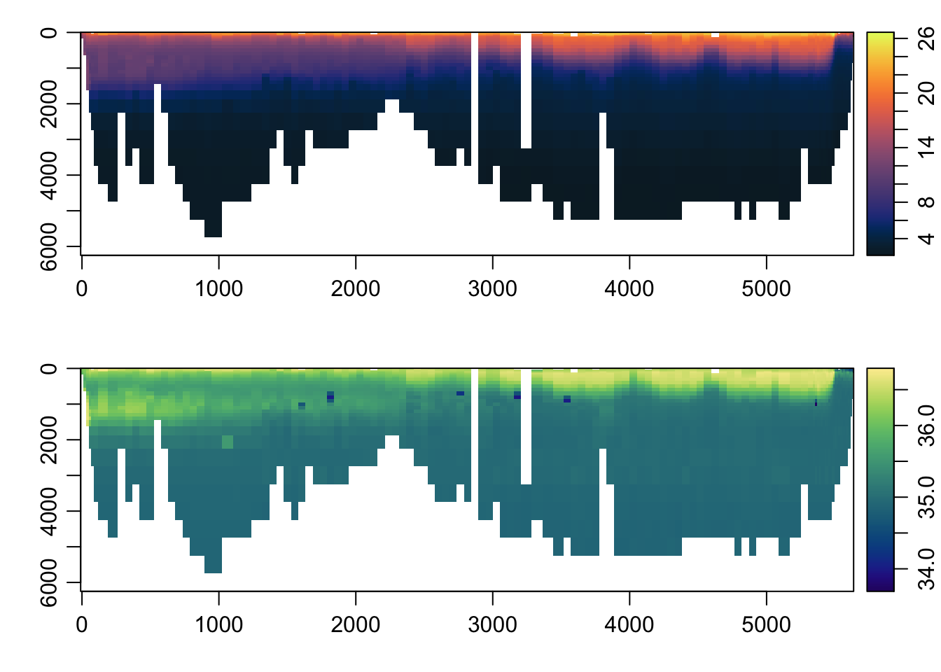

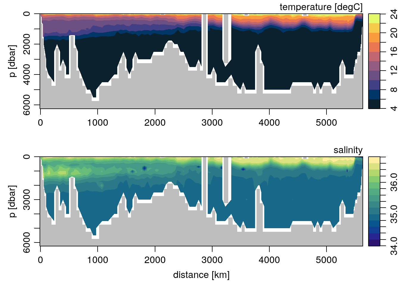
Or we can do some fancier things, like use the colormap() function and plot some filled contours:

par(mfrow=c(2, 1))
Tcm <- colormap(T, breaks=seq(4, 24, 2), col=oceColorsTemperature)
Scm <- colormap(S, breaks=seq(34, 36.8, 0.2), col=oceColorsSalinity)
imagep(distance, p, T, colormap=Tcm, flipy=TRUE,
       ylab='p [dbar]', filledContour=TRUE,
       zlab='temperature [degC]')
imagep(distance, p, S, colormap=Scm, flipy=TRUE,
       xlab='distance [km]', ylab='p [dbar]', filledContour=TRUE,
       zlab='salinity')

Making nice plots of the sections themselves

Finer control over the section plot

Related Articles