Calculating buoyancy frequency for argo/section objects using the apply() family

Buoyancy frequency

The definition of $N^2 $ is:

\[ N^2 = \frac{-g}{\rho} \frac{\partial \rho}{\partial z} \]

where \(g\) is the acceleration due to gravity, \(\rho = \rho(z)\) is the fluid density, and $z $ is the vertical coordinate. Essentially $N^2 $ describes the vertical variation of fluid density (also known as “stratification”).

Calculating \(N^2\) for regular ctd objects is easily accomplished with the function oce::swN2(). A caution: readers are encouraged to read the documentation carefully, as the details of the actual calculation can have important consequences when applied to real ocean data.

\(N^2\) for station objects

For the case of a station object (which is essentially a collection of ctd stations), the most straightforward way to calculate \(N^2\) is to use the lapply() function to “apply” the swN2() function to each of the stations in the object. An example:

library(oce)
data(section)
section[['station']] <- lapply(section[['station']],
                               function(x) oceSetData(x, 'bvf', swN2(x)))

The line with the lapply() command takes the list of stations from the section object, and evaluates each of the resulting ctd objects using the oceSetData() function to add the result of swN2() back into the station @data slot.

If we wanted to make a nice plot of the result, we could do:

col <- colorRampPalette(c('white', rev(oceColorsViridis(32))))
plot(section, which='bvf', ztype='image', zbreaks=seq(0, 1e-4, 0.5e-5), zcol=col)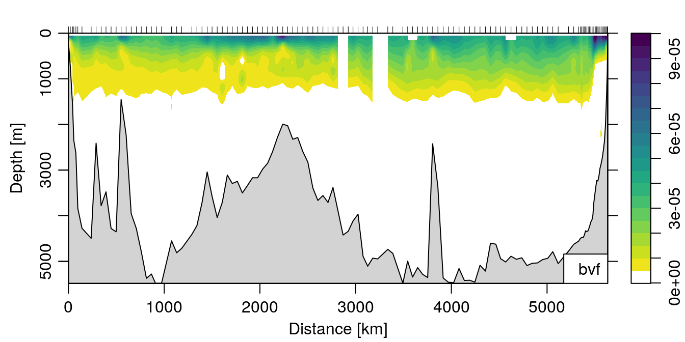

where I’ve defined a custom colormap just for the fun of it.

\(N^2\) for argo objects

In an argo object, the default storage for the profiles is a matrix, rather than a list of ctd objects. To calculate \(N^2\) and make a plot, the simplest approach would be to use as.section() to convert the argo object to a section class object and then do as above. However, having the field as a matrix allows for greater flexibility in plotting, e.g. using the imagep() function, so one might want to calculated \(N^2\) in a manner consistent with the default argo storage format.

Let’s load some example data from the argo dataset included in oce:

data(argo)
argo <- argoGrid(argo)

Note that I’ve gridded the argo fields so the matrices are at consistent pressure levels. Now we create a function that can be applied to each of the matrix columns, to calculate \(N^2\) from a single column of the density matrix:

N2 <- function(x) {
    swN2(argo[['pressure']][,1], x)
}

Now we use the above function N2 to calculate buoyancy frequency and add it back to the original object, like:

argo <- oceSetData(argo, 'N2', apply(swSigmaTheta(argo), 2, N2) )

Note that because of the difference between the “list” and “matrix” approach, the oceSetData() occurs outside of the apply(). Also note the second argument in the apply() call, which specifies to apply the N2() function along the 2nd dimension of the density matrix, i.e. along columns.

Now, lets make a sweet plot of the N2 field using imagep()!

p <- argo[['pressure']][,1]
t <- argo[['time']]
imagep(t, p, t(argo[['N2']]), flipy=TRUE, col=col, breaks=seq(0, 1e-4, 1e-6),
       ylab='pressure [dbar]',
       zlab=expression(N^2~group('[', 1/s^2, ']')), zlabPosition = 'side',
       mar=c(3, 3, 2, 0.5))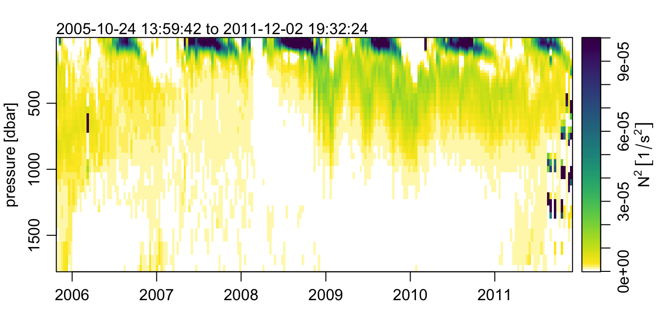

A thing of stratified beauty, if I do say so myself.