Using the oce package to make nice maps

2019-07-12 in OCE • R
plot maps proj coastline arctic
4 min read

Introduction

Making maps is a pretty important part of doing, and presenting, ocean data analyses. Except for very small domains, using map projections is crucial to ensure that the map is not distorted. This is particularly true for polar and high latitude regions, such as the Arctic (where I do much of my work).

In this post I will give a brief introduction to making projected maps with the oce package, including not just the land/coastline but also various ways of plotting the bathymetry. For the latter I will discuss the handy marmap package.

Making a polar stereographic map of the Canadian Arctic

To make “projected” maps with oce, you can use the mapPlot() function. The easiest way is to use mapPlot() with a coastline object, to set the projection you want, and then add other elements (such as bathymetry, etc) using functions like mapLines(), mapPoints(), mapImage(), etc. You may need to redo the coastline at the end to clean up anything that might have plotted over land that you don’t want.

The coastlineWorldFine dataset from the ocedata package is pretty good for sub-regions such as the Canadian Arctic.

library(oce)

## Loading required package: gsw

## Loading required package: testthat

library(ocedata) #for the coastlineWorldFine data
data(coastlineWorldFine)

To get the projection you want, it must be passed in the projection= argument using “proj4” syntax as a character string. You can read up on the syntax and available projection in the help – i.e. ?mapPlot, or have a look at:

[PROJ4]https://proj.org/operations/projections/index.html)

For polar maps, the most commonly used is the stereoraphic projection:

## Save it to a function to make it easy to re-run
mp <- function() {
    mapPlot(coastlineWorldFine, projection="+proj=stere +lon_0=-90 +lat_0=90",
            longitudelim = c(-120, -60),
            latitudelim = c(60, 85), col='grey')
}
mp()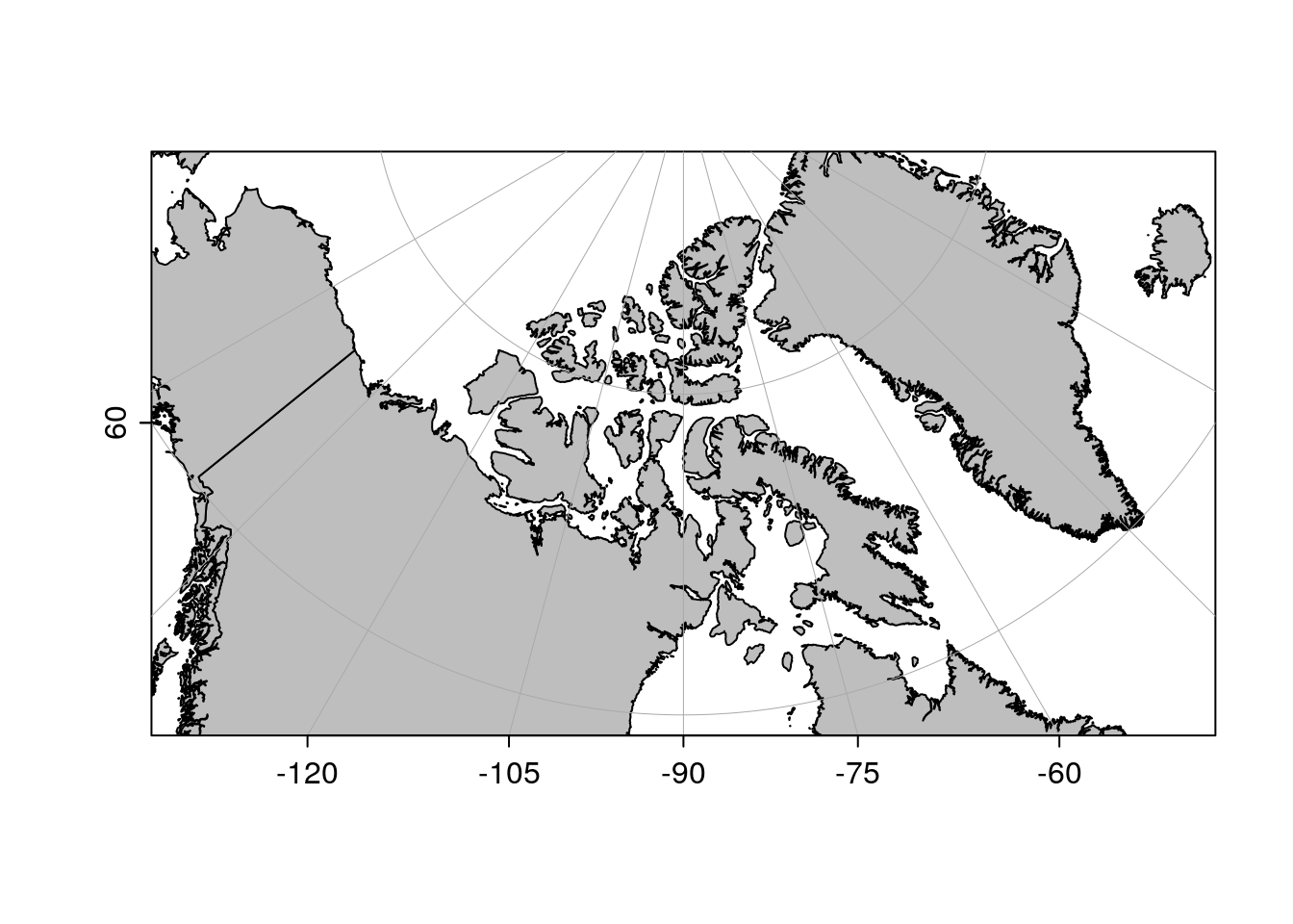

In this example, the +lon_0 parameter defines the longitude at the center of the projection, and the +lat_0 is the latitude at the center of the projection. The mapPlot() arguments longitudelim and latitudelim are used to control the extent of the map.

As for adding bathymetry, there are a few options:

oce includes a low-res version of the etopo dataset, called topoWorld that can be used, either as a contour plot or as an image plot.
The marmap package allows easy downloading of subsets of the full resolution etopo data, which can be used to make nicer plots. One downside is that because of the “triangle” nature of a polar stereoraphic projection you have to download a lot more data than you really need.

Using `topoWorld`

A quick way of adding bathymetry is to simply use the mapContour() function (analogous to the base-R contour()).

data(topoWorld)
mp()
mapContour(topoWorld, levels=-c(500, 1000, 2000, 4000),
           drawlabels=FALSE)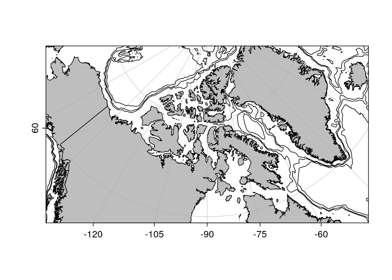

Contour plots can be tricky, because of the labeling etc, and choosing which contours to plot. Another option is to use the mapImage() function:

mp()
mapImage(topoWorld, col=oceColorsGebco, breaks=seq(-4000, 0, 500))
mapPolygon(coastlineWorldFine, col='grey')
mapGrid()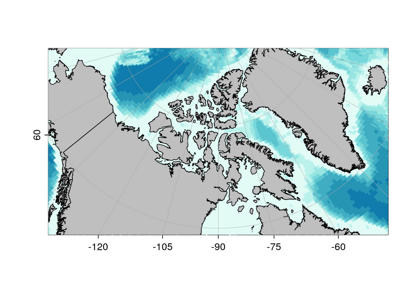

But sometimes using mapImage() shows off the “blockiness” of the low-res topoWorld dataset – especially near the poles where the shape of the cells (evenly divided in lon/lat space) gets really skinny.

One fix is to use a higher res data set (so the “boxes” are smaller – see next section). Another is to use the fillContour argument in mapImage() to plot filled contours rather than the individual grid cells.

mp()
mapImage(topoWorld, col=oceColorsGebco, breaks=seq(-4000, 0, 500), filledContour = TRUE)
mapPolygon(coastlineWorldFine, col='grey')
mapGrid()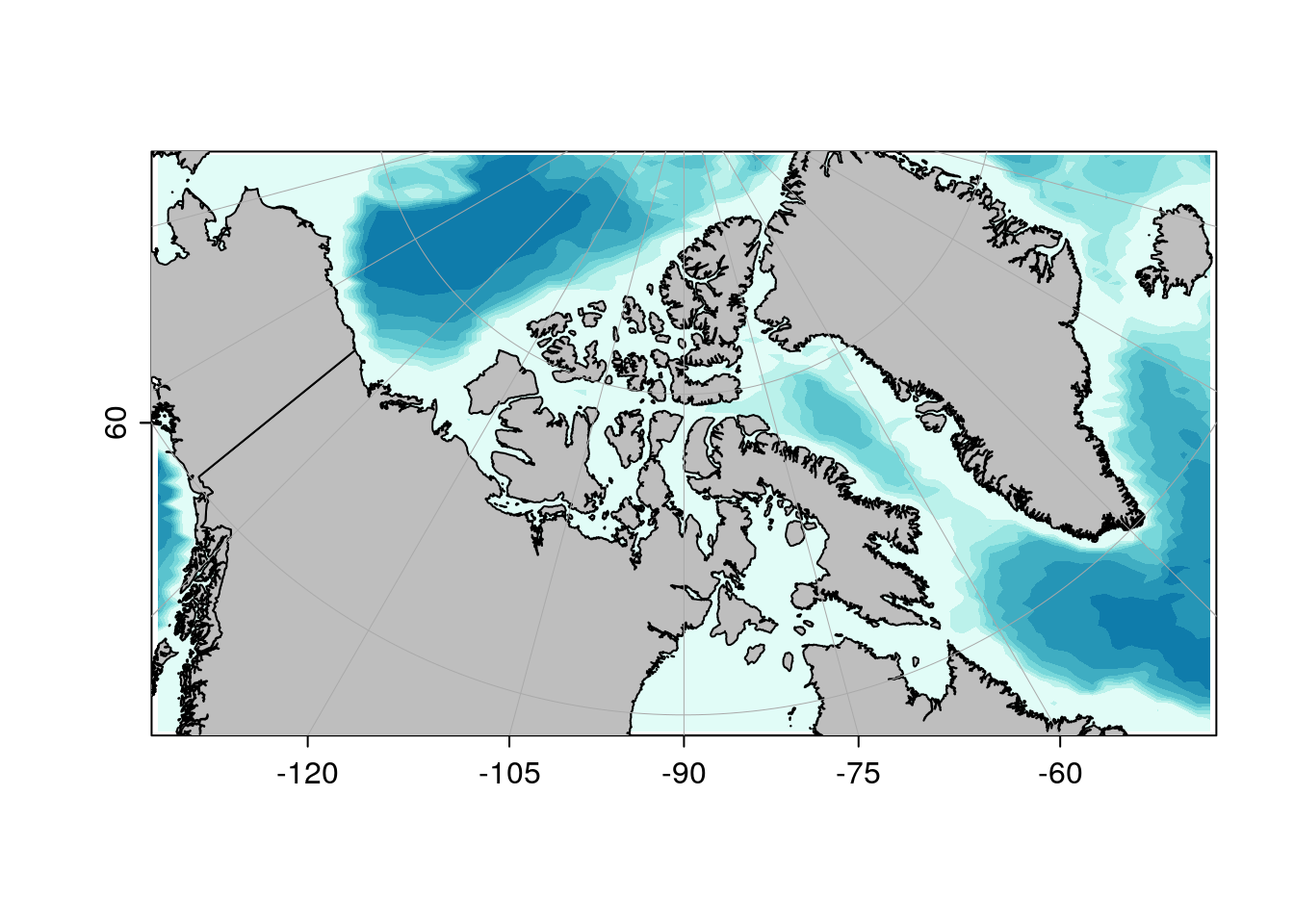

Using marmap

Here we load the marmap package and download the bathymetry. Note that because we have the North Pole in view, we basically have to download an entire half hemisphere. It takes a little while to download, but if you use the keep=TRUE argument then it will just reload it from the file each time.

However, because there is so much more data, the plotting can be quite a bit slower.

library(marmap)

## Registered S3 methods overwritten by 'adehabitatMA':
##   method                       from
##   print.SpatialPixelsDataFrame sp  
##   print.SpatialPixels          sp

## 
## Attaching package: 'marmap'

## The following object is masked from 'package:oce':
## 
##     plotProfile

## The following object is masked from 'package:grDevices':
## 
##     as.raster

b <- as.topo(getNOAA.bathy(-180, 0, 55, 90, keep=TRUE))

## File already exists ; loading 'marmap_coord_-180;55;0;90_res_4.csv'

mp()
mapImage(b, col=oceColorsGebco, breaks=seq(-4000, 0, 500))
mapPolygon(coastlineWorldFine, col='grey')
mapGrid()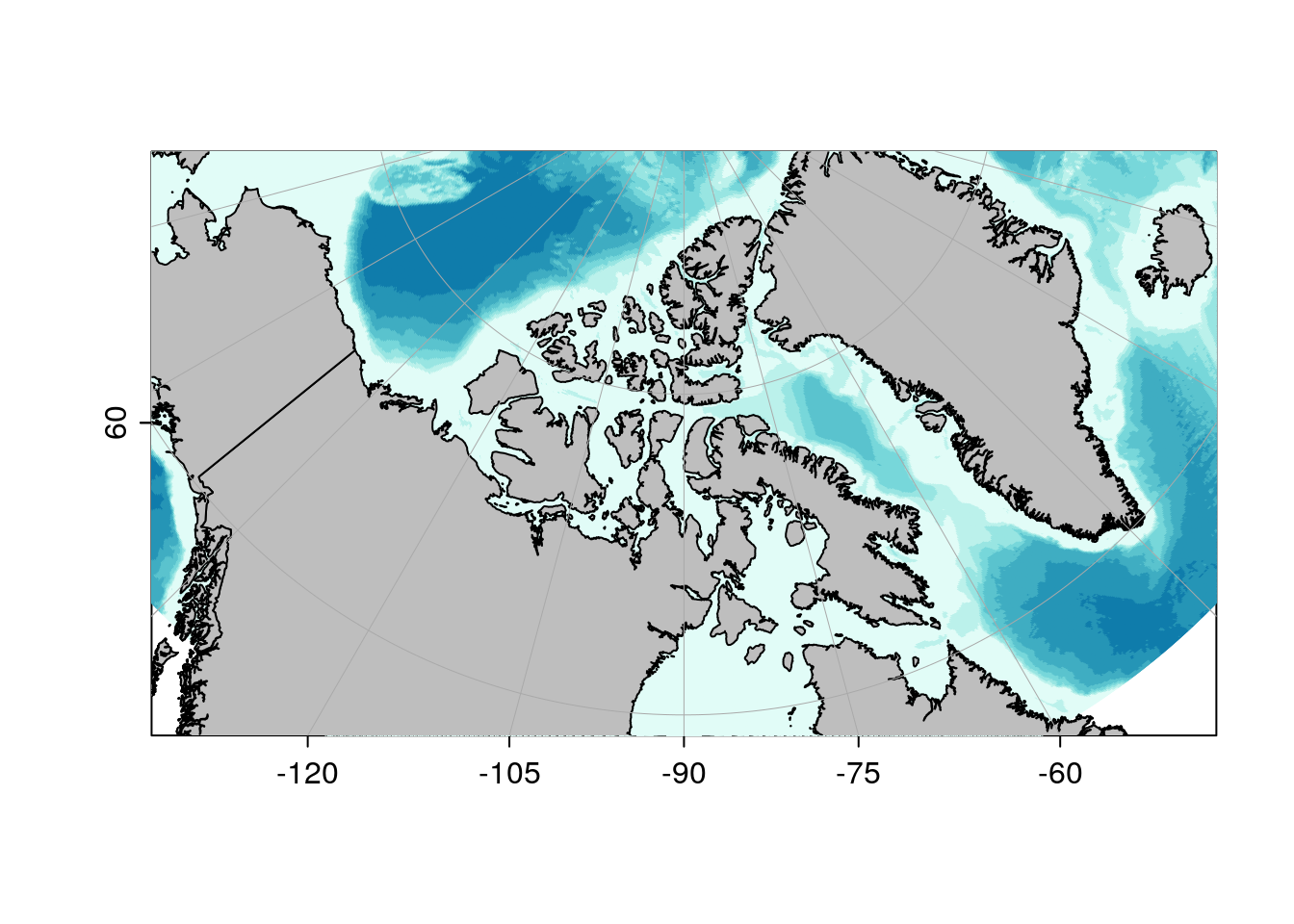

Looks pretty good, though!

Introduction

Making a polar stereographic map of the Canadian Arctic

Using topoWorld

Using marmap

Related Articles

Using `topoWorld`