Recording and replaying plots with the `recordPlot()` function

R plot systems

First, for those who either don’t use R or who have been living under a rock, there are (in my opinion) two major paradigms for producing plots from data in R. The first is the original “base graphics” system – the sequence of functions bundled with R that are part of the graphics package which is installed and loaded by default.

The second is the ggplot2 package, written by Hadley Wickham, which uses the “grammar of graphics” approach to plotting data and is definitely not your standard plot(x, y) approach to making nice-looking plots. To be fair, I think ggplot is quite powerful, and I never discourage anyone from using it, but because I don’t use it in my own work (for many reasons too complicated to get into here) I don’t tend to actively encourage it, either.

Storing ggplots in objects

Anyway, one thing that I’ve always liked about the ggplot approach is that the components of the plot can be saved in objects, and built up in pieces by simply adding new plot commands to the object. A typical use case might be like this (using the built-in iris dataset):

library(ggplot2)
ggplot(iris, aes(x=Sepal.Length, y=Petal.Length)) + geom_point()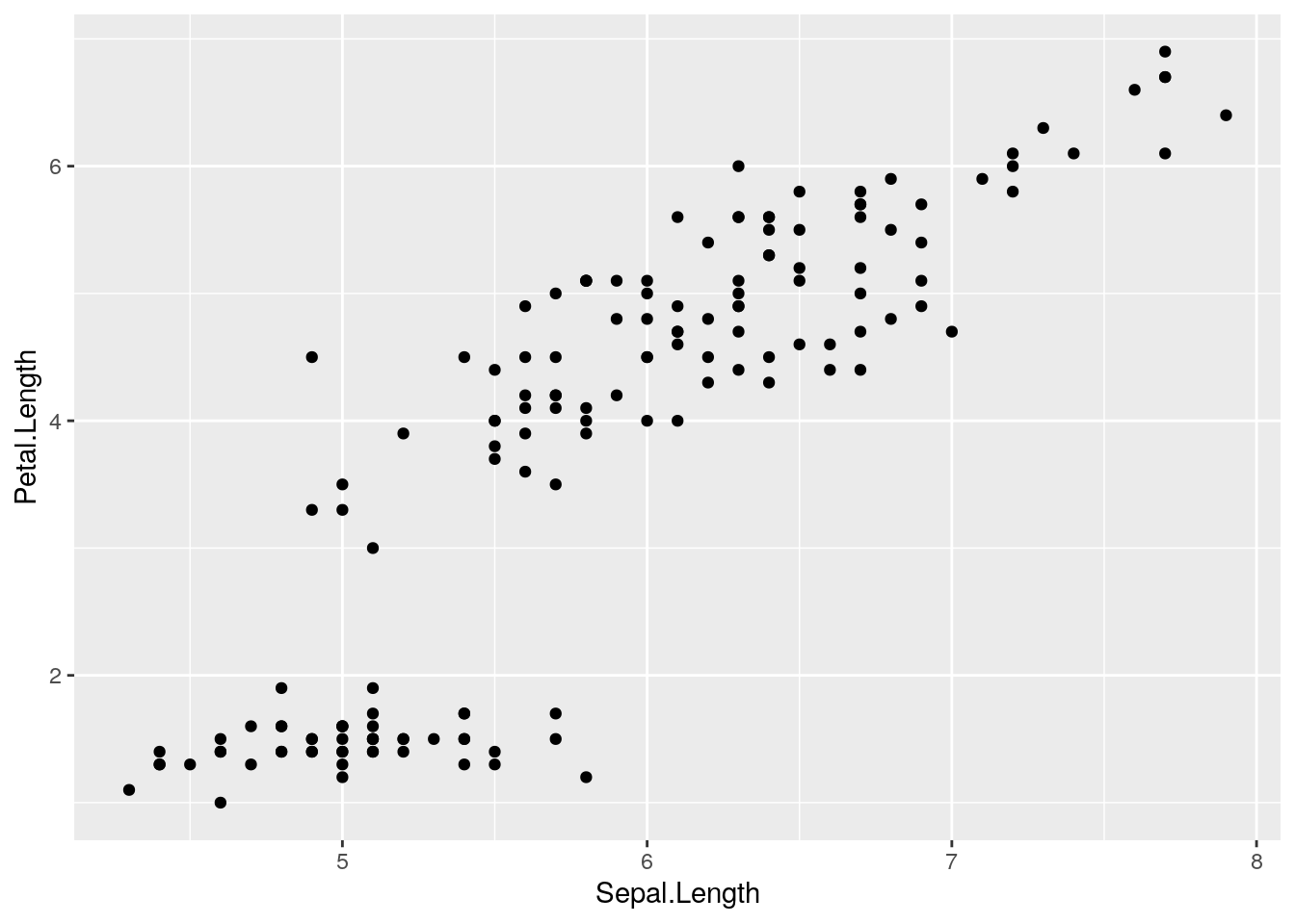

Note how the foundation of the plot is created with the ggplot() function, but the points are added though the + of the geom_point() function.

However, for more complicated plots, the components are often saved into an object which can have other geom_* bits added to it later on. Then the final plot is rendered by “printing” the object:

pl <- ggplot(iris, aes(x=Sepal.Length, y=Petal.Length))
pl <- pl + geom_point() # add the points
pl <- pl + geom_density2d() # add a 2d density overlay
pl # this "prints" the plot and renders it on the screen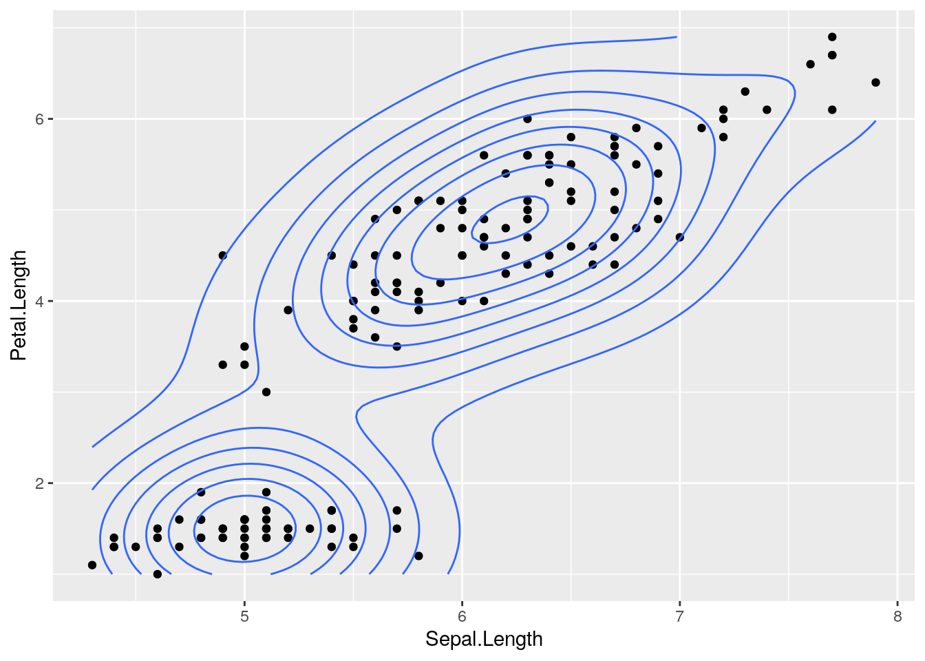

Admittedly, this is pretty cool, not the least of which because you can always re-render the plot just by printing the object.

Recording a base graphics plot

While not quite the same, I recently discovered that it’s possible to “record” a base graphics plot to save in an object, allowing you to re-render the same plot. The case that led me to stumble onto this was where I had a complicated bit of code that made a plot that fit a model to data, and then I wanted to step through various iterations of removing certain points, adding new ones, to see what the effect on the fit would be.

I often do this using the pdf() function in R, so that each new plot can become another page in the pdf file that can be stepped through. However, another use case that I thought of after is in writing Rmarkdown documents (like this one!), where you’d like to keep showing a base plot but add different elements to it consecutively. Because of the way Rmarkdown works, the graphics from each code chunk are rendered independently, so it’s not possible to say, generate a plot in one chunk (using plot()), and then add to it with points() or lines() in another chunk.

Let’s see an example. I’ll make a plot that has a bunch of pieces, and then save it to an object with recordPlot():

plot(iris$Sepal.Length, iris$Petal.Length,
     xlab='Sepal Length', ylab='Petal Length',
     pch=round(runif(nrow(iris), max=25)))
grid()
title('My base plot')

pl <- recordPlot()

Now, if I want to redo the plot exactly as I already did, I just “print” the object:

pl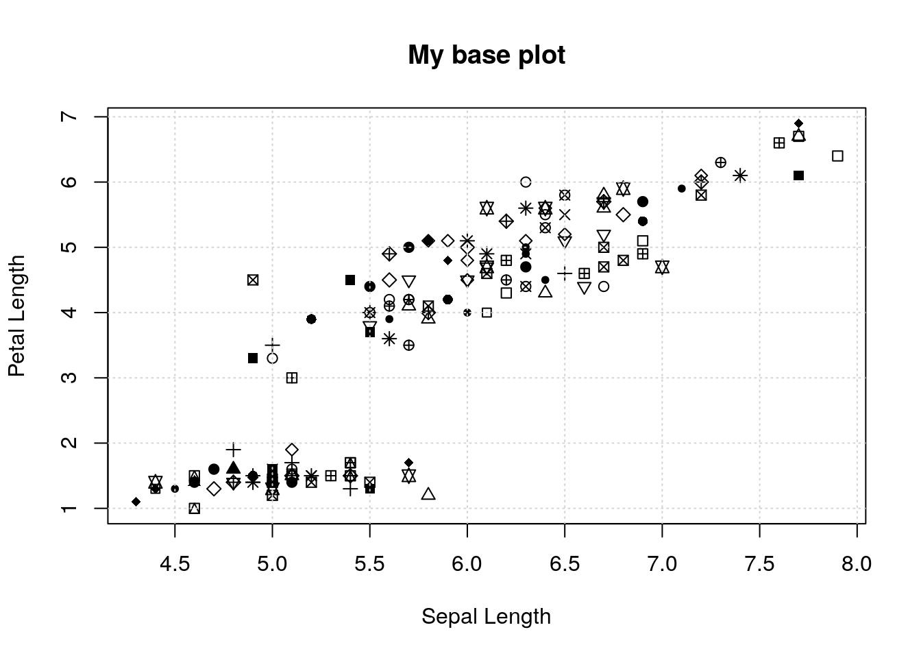

So now if I want to redo the plot, but add different pieces, I can redo the plot as above, and add whatever I want with the normal base graphics functions:

pl # start with the original plot
m <- lm(Petal.Length ~ Sepal.Length, data=iris)
abline(m, lwd=2, col=2)
title(c('', '', 'with a subtitle!'), col.main=2)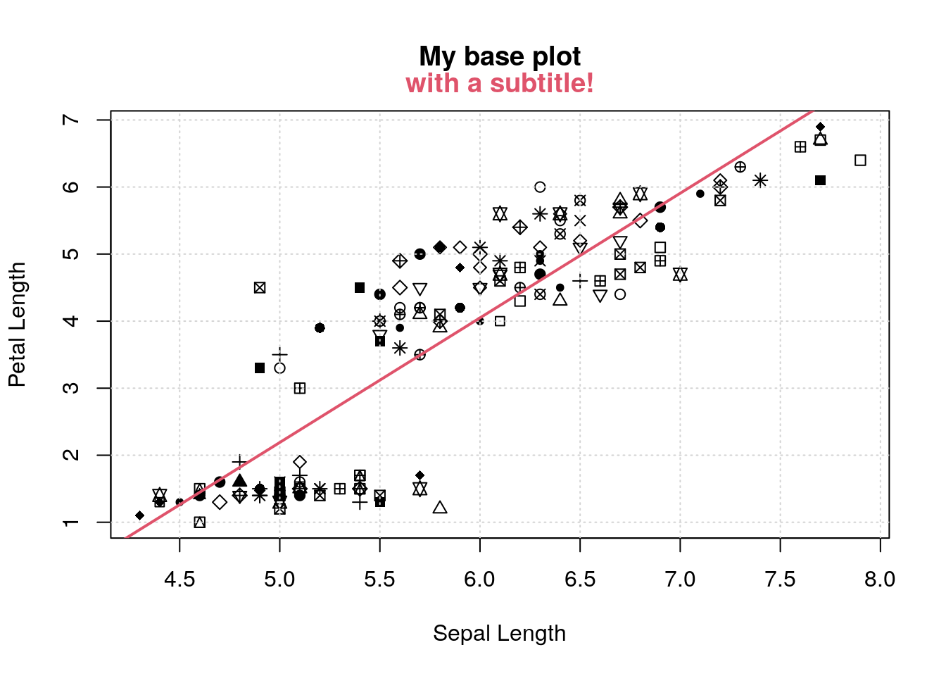

pl <- recordPlot()

And to keep going I just keep recording the plot and starting each chunk with it:

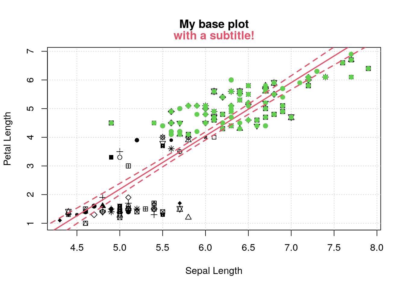
pl
II <- iris$Petal.Length > 4
points(iris$Sepal.Length[II], iris$Petal.Length[II], col=3, pch=19)
sl <- seq(4, 8, length.out=100)
pl <- predict(m, newdata=list(Sepal.Length=sl), interval='confidence')
lines(sl, pl[,2], lty=2, col=2, lwd=2)
lines(sl, pl[,3], lty=2, col=2, lwd=2)