Introduction

Tidal analysis is something that oceanographers do a lot of. Tides occur just about everywhere, to varying degrees and with varying astronomical forcings (sun, moon, etc), and aside from wanting to study the tides themselves, often we want to get rid of the tidal signal from some data so that we can look at the oceanographic processes occuring underneath.

Tidal harmonic analysis is a technique that has been around for some time (see Foreman et al (2009)¹ for a nice review, as well as Godin (1972)² and Foreman (1977)³ as canonical references). I won’t get into the details here, but the basic premise is that we fit sinusoids of a known frequency (e.g. the astronomical forcings) to a time series, to determine an amplitude and phase for each constituent. The simplest version of this is applied to a time series of sea level height (or pressure), where the high/low tides correspond to the interaction of each of the frequencies that contribute to the tidal variations at that location.

Harmonic Analysis of currents

While the tidal forcing causes sea level to go up and down (according to the prescribed constituent frequencies), the result in the ocean is that there are also currents driven by the tidal variations. Because (horizontal) currents are not a scalar (i.e. 1D) time series, the above approach using tidem() can only be applied by separately considering a harmonic analysis of the “u” and “v” (e.g. east/west and north/south) velocity components. A more common approach, using the classical fitting method of least squares, is to combine the horizontal velocity components into a single complex velocity, e.g.

\[ U(t) = u(t) + i v(t) \]

where the results of the analysis now describe the combined fit of the two related components. A common summary result from such a fit is to describe a “tidal ellipse”, which is a horizontal ellipse that would be traced out by each of the tidal constituents – the major and minor axes of the ellipse describe the size of the two orthonal components and the phases of the u/v oscillations determine an ellipse “orientation”, or angle.

The oce package, due to the use of lm(), is not able to perform a complex analysis. However, the python package Utide can do this analysis, and thanks to the reticulate package in R it is easy to run both R and python code simultaneously, while passing variables back-and-forth between the two systems.

Setting up a python environment to do tidal analysis

There are many different ways to set up and configure a python environment for doing oceanography. I am not a python expert, so take any of my advice with a grain of salt, but other competent oceanographers that I know that use python seem to prefer the “miniconda” distribution, which uses conda as a package manager (and can also use the more development-oriented package repository of conda-forge).

Whenever I am setting up a new miniconda install, I use the instructions provided by the University of Hawaii Currents group, found here. For completeness here I’ll just repeat the steps as I have followed them. The install is nearly identical on both MacOS and Linux. I have not had the opportunity to try the full install on a normal Windows OS, because even on Windows I use the Windows Subsystem for Linux (WSL) for all my scientific coding (essentially just a terminal Ubuntu installation embedded in Windows).

Copied directly from the above UH page, follow below to install the python miniconda environment:

Install Miniconda base

To begin, install the current 64-bit Python 3 Miniconda base that matches your operating system. We will use the shell script version (*.sh) of the installer, not a GUI version (*.pkg on the Mac). We don’t even need a browser to download the installer. Open a terminal window so you can run commands. Then you can download the Mac installer by executing:

curl -O https://repo.anaconda.com/miniconda/Miniconda3-latest-MacOSX-x86_64.sh

if your machine has an Intel processor, or:

curl -O https://repo.anaconda.com/miniconda/Miniconda3-latest-MacOSX-arm64.sh

if you have a machine with the M1 or M2 chip (“Apple Silicon”, which uses the ARM architecture).

For Linux:

curl -O https://repo.anaconda.com/miniconda/Miniconda3-latest-Linux-x86_64.sh

After downloading, use the bash interpreter to execute the shell script, like this:

bash Miniconda3-latest-MacOSX-x86_64.sh

but substituting the corresponding file name if you are on Apple Silicon or Linux. Do not use “sudo”; execute the script as a normal user, and let the installation occur in the default location in your home directory. Use the spacebar to page down through the user agreement, hit return, and “yes” to accept it. I suggest answering “no” to:

Do you wish the installer to initialize Miniconda3
by running conda init? [yes|no]

We will take care of this manually in a minute, when the installer has finished.

Are you running zsh, or bash? If you are on Linux, it is almost certainly bash. If you are on an older Mac, it might be bash. If you are on a newer Mac, with Catalina or later, it is probably zsh. The banner at the top of the Mac terminal window will show which one you are using. You can also get a list of processes you are running in the terminal, including either bash or zsh, by executing:

ps

If it says “-bash”, ignore the hyphen; it is just bash. If you are running zsh, then execute, on the command line:

~/miniconda3/bin/conda init zsh

or if you are running bash:

~/miniconda3/bin/conda init bash

Either way, this command will tell you that it is modifying a file, “.zshrc” or “.zprofile” if you are running zsh, and otherwise either “.bash_profile” or “.bashrc”. Note the name of the file being modified; you might need it later.

Next, put some configuration entries in your .condarc file by cutting and pasting the following lines into your terminal. (The backslashes are line continuations.) You might need to hit “return” after pasting, so the last command will be executed:

~/miniconda3/bin/conda config --add channels conda-forge
~/miniconda3/bin/conda config --set channel_priority strict
~/miniconda3/bin/conda config --set auto_activate_base false
~/miniconda3/bin/conda config --append create_default_packages ipython \
         --append create_default_packages pip \
         --append create_default_packages "blas=*=openblas"

(I am recommending a subset of the configuration options described in https://gist.github.com/ocefpaf/863fc5df6ed8444378fbb1211ad8feb1.)

Now quit the terminal application completely (this is necessary with OSX; on Linux you only need to close the terminal window and open a new one), restart it, and check that the conda executable is found. Execute:

which conda

Depending on the shell you are running, it should return either a path that starts with your home directory followed by miniconda3/condabin/conda (if running bash), or multiple lines of shell code defining a conda function (if running zsh).

Making a conda environment for tidal analysis

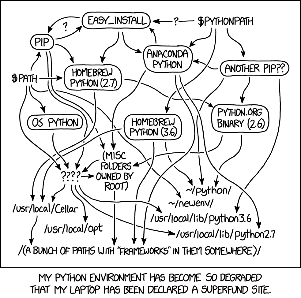
At this point, the next step is simply to create conda “environments” that can be used to write/run python code. The environment approach to containerizing workflows is somewhat foreign to the R world, but fairly standard in python. To be honest, I like the simplicity of the R package ecosystem, though I do see the advantages to keeping python environments associated with projects and avoiding something that looks like this (from XKCD):

XKCD python environments

To create an environment that can be used for tidal analysis, I did the following:

conda create -n tides utide pandas

which creates a conda environment called “tides” into which it installs the packages “utide” and “pandas” (needed for some R to python date conversions) and their dependencies.

Note that if you intend to use this environment from the command line (e.g. by starting python, or a python IDE such as Jupyter), it is necessary to “activate” the environment by doing:

conda activate tides

To use this environment in an R script, this isn’t necessary.

Using reticulate to run the Utide python package in R

Now that all the python requirements are installed, we can call the package through R using the reticulate package. First, we load the libraries and set the conda environment that we want to use for reticulate:

library(oce)

## Loading required package: gsw

library(reticulate)
use_condaenv("tides")

The functions associated with the python libraries can be loaded into the R workspace with the import() function, like:

utide <- import("utide")
pandas <- import("pandas")
np <- import("numpy")

and we can load the example “tidalCurrent” dataset included in oce:

data(tidalCurrent)
t <- tidalCurrent$time
u <- np$array(tidalCurrent$u)
v <- np$array(tidalCurrent$v)
tpy <- pandas$to_datetime(as.numeric(t), unit = "s", utc = TRUE)

The last line converts the R POSIX format time to a pandas “datetime”, needed for Utide.

We can then perform the tidal analysis using the Utide coef() function:

coef <- utide$solve(tpy, u, v,
    lat = 45, nodal = FALSE, trend = FALSE, method = "ols",
    conf_int = "linear", Rayleigh_min = 0.95
)

## solve: matrix prep ... solution ... done.

which produces a list coef that has fields:

names(coef)

##  [1] "aux"      "diagn"    "g"        "g_ci"     "Lsmaj"    "Lsmaj_ci"
##  [7] "Lsmin"    "Lsmin_ci" "name"     "nI"       "nNR"      "nR"      
## [13] "PE"       "SNR"      "theta"    "theta_ci" "umean"    "vmean"   
## [19] "weights"

Making a tidal prediction based on the fit, is as easy as using the utide reconstruct() function:

tide <- utide$reconstruct(t = tpy, coef = coef)

## prep/calcs ... done.

Let’s make some plots to show that it works!

par(mfrow = c(2, 1))
oce.plot.ts(t, u)
lines(t, tide["u"], col = 2)
legend("bottomleft", c("data", "fit"), lty = 1, col = 1:2, bg = "white")
oce.plot.ts(t, v)
lines(t, tide["v"], col = 2)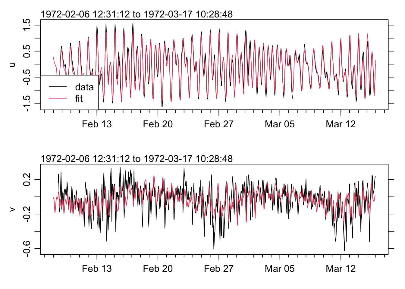

We can visualize the tidal constituent ellipses, by first creating a function that will draw an ellipse, and then looping through the constituents from the fit and adding them to a hodograph of the currents:

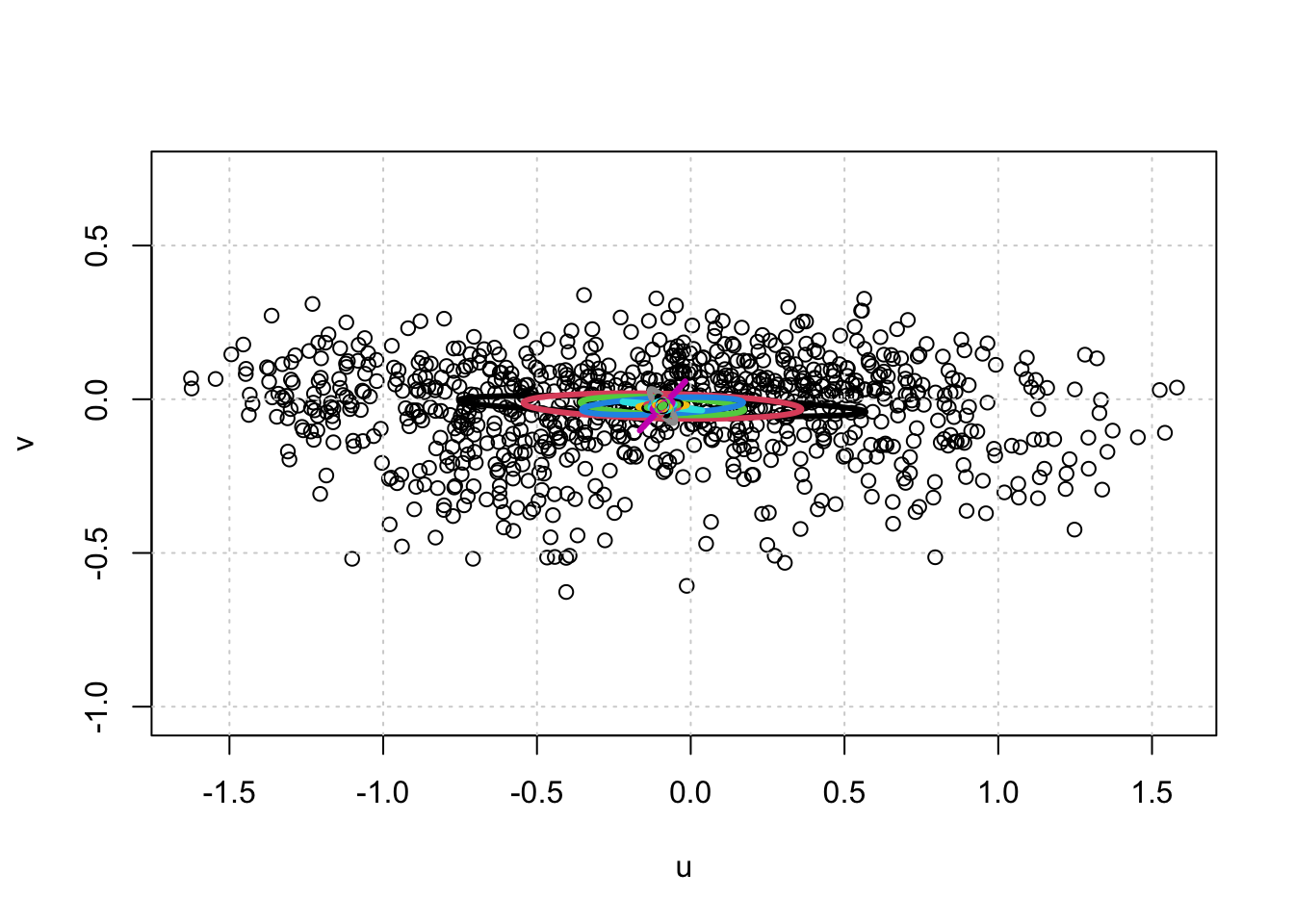
ellipse <- function(xc = 0, yc = 0, Lmaj, Lmin, phi, ...) {
    th <- seq(0, 2 * pi, 0.01)
    x <- xc + Lmaj * cos(th) * cos(phi) - Lmin * sin(th) * sin(phi)
    y <- yc + Lmaj * cos(th) * sin(phi) + Lmin * sin(th) * cos(phi)
    lines(x, y, ...)
}
par(mfrow = c(1, 1))
plot(u, v, asp = 1)
grid()
for (i in seq_along(coef$name)) {
    ellipse(coef$umean, coef$vmean, coef$Lsmaj[i], coef$Lsmin[i], coef$theta[i] * pi / 180, lwd = 3, col = i)
}