
Introduction
Making plots in oceanography (or anything, really) often requires creating some kind of “color map” – that is, having a color represent a field in a plot that is otherwise two-dimensional. Frequently this is done when making “image”-style plots (known in MatlabTM parlance as “pcolor” or pseudocolor plots), but could also be in coloring points on a 2D scatter plot based on a third variable (e.g. a TS plot with points colored for depth).
There are a whole bunch of different ways to make colormaps in R, including various approaches that are derived from the “tidyverse” and ggplot2 package for analyzing and plotting data. I don’t really use that approach for most of my work, so won’t touch on them here.
Instead, the purpose of this post (inspired by a question from a colleague who I know is a Matlab and Python user) is to show some of the ways various functions contained in the oce package cab be used to make colormaps and colorbars (or “palettes”). In particular, for the case where one wants a “discrete” (i.e. not continuous) colormap.
The imagep() function
For making image-style plots, the function imagep() provided by the oce package is a handy function for quickly making nice-looking pseudocolor plots of matrices. The “p” in imagep() stands for “palette” or “pseudocolor”. Mostly, it is a wrapper around the base R function image(), to allow for increased control of the axes, colors, and palette specification.
library(oce)## Loading required package: gsw## Loading required package: testthatlibrary(ocedata)
library(cmocean)
data(levitus)
par(mfrow=c(1, 3))
with(levitus, imagep(longitude, latitude, SST))
with(levitus, imagep(longitude, latitude, SST, col=oceColorsJet, breaks=-2:25))
with(levitus, imagep(longitude, latitude, SST, col=cmocean('thermal'), breaks=seq(-2, 30, 2)))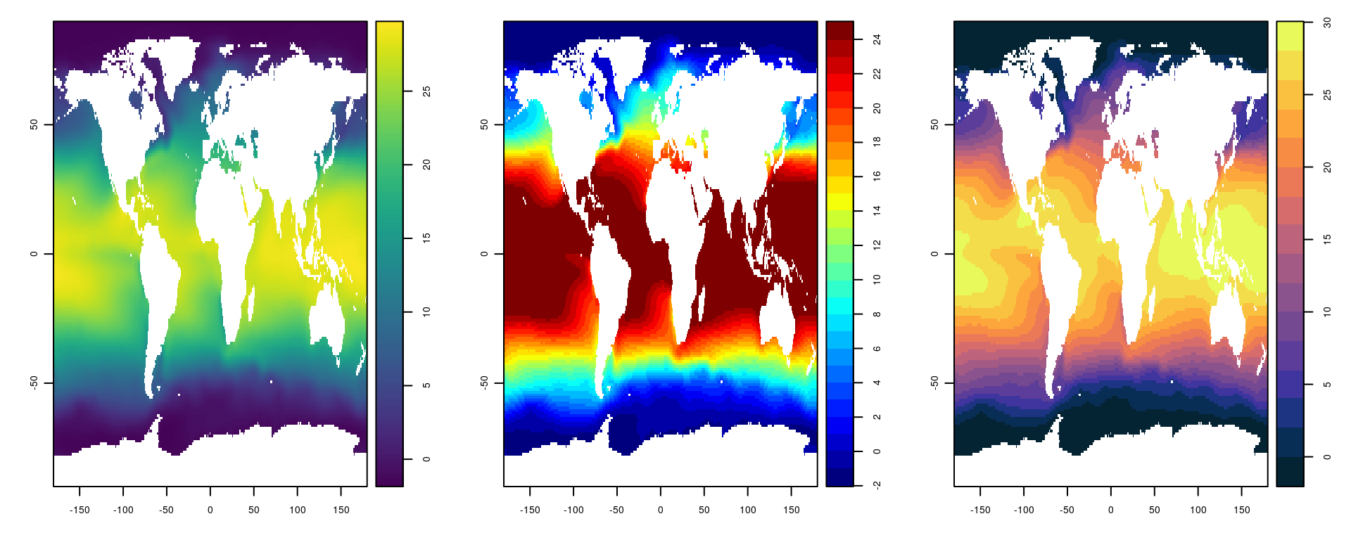
The above example shows how to use imagep() with 3 different colormaps (the default, the classic “jet” scheme, and the cmocean package) to generate an image plot with a nice palette automatically placed on the side.
The drawPalette() and colormap() functions
Under the hood, the imagep() function calls another function to actually draw the palette on the side of the plot – the drawPalette() function. That function can be called on it’s own, enabling plot building to be much more flexible. Additionally there is the colormap() function, which allows for detailed specification of the colormap properties to use, which can then be passed as an object to drawPalette().
For example, say we wanted to make a TS (temperature-salinity) plot of the Levitus surface data, but with each point colored by latitude in 10 degree increments. We do that first by making a colormap object:
cm <- colormap(expand.grid(levitus$latitude, levitus$longitude)[,1], breaks=seq(-90, 90, 10), col=oceColorsViridis)(note that we use expand.grid() to make the number of lon/lat points match the matrices).
Looking inside the object, we can see some of the details that further plotting/palette functions can make use of:
str(cm)## List of 11
## $ zlim : num [1:2] -90 90
## $ breaks : num [1:19] -90 -80 -70 -60 -50 -40 -30 -20 -10 0 ...
## $ col : chr [1:18] "#440154" "#481769" "#472A7A" "#433D84" ...
## $ zcol : chr [1:64800] "#440154" "#440154" "#440154" "#440154" ...
## $ missingColor: chr "gray"
## $ x0 : num [1:18] -80 -70 -60 -50 -40 -30 -20 -10 0 10 ...
## $ x1 : num [1:18] -80 -70 -60 -50 -40 -30 -20 -10 0 10 ...
## $ col0 : chr [1:18] "#440154" "#481769" "#472A7A" "#433D84" ...
## $ col1 : chr [1:18] "#440154" "#481769" "#472A7A" "#433D84" ...
## $ zclip : logi FALSE
## $ colfunction :function (z)
## - attr(*, "class")= chr [1:2] "list" "colormap"Some of those fields are obvious (some probably aren’t to inexperienced users) but one field that is handy to know about is the zcol field. This encodes a color for every value in the original object based on the colormap specification. So, we can make a plot with the points colored based on the colormap using the argument col=cm$zcol. We can also add the palette to the plot using the drawPalette() function, which has to be called before the main plot:
drawPalette(colormap=cm)
plotTS(with(levitus, as.ctd(SSS, SST, 0)), pch=19, col=cm$zcol, mar=par('mar'))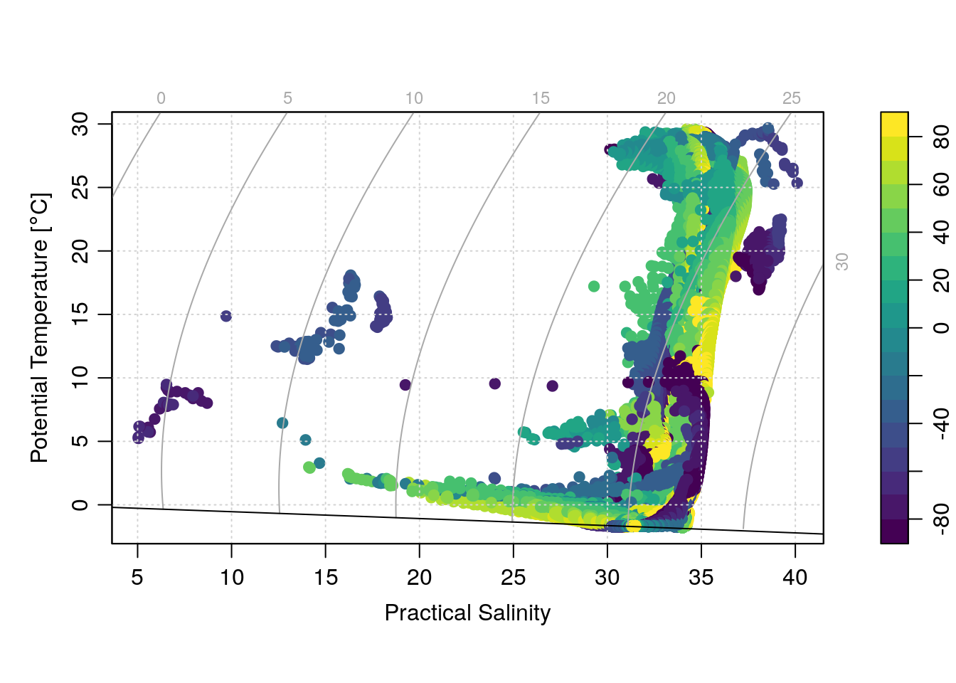
One problem that can happen when there are a lot of points is that overplotting obscures patterns in the colors. An easy way to fix this is to randomize the order of the plotted points with the sample() function:
drawPalette(colormap=cm)
sI <- sample(seq_along(cm$zcol))
plotTS(with(levitus, as.ctd(SSS[sI], SST[sI], 0)), pch=19, col=cm$zcol[sI], mar=par('mar'))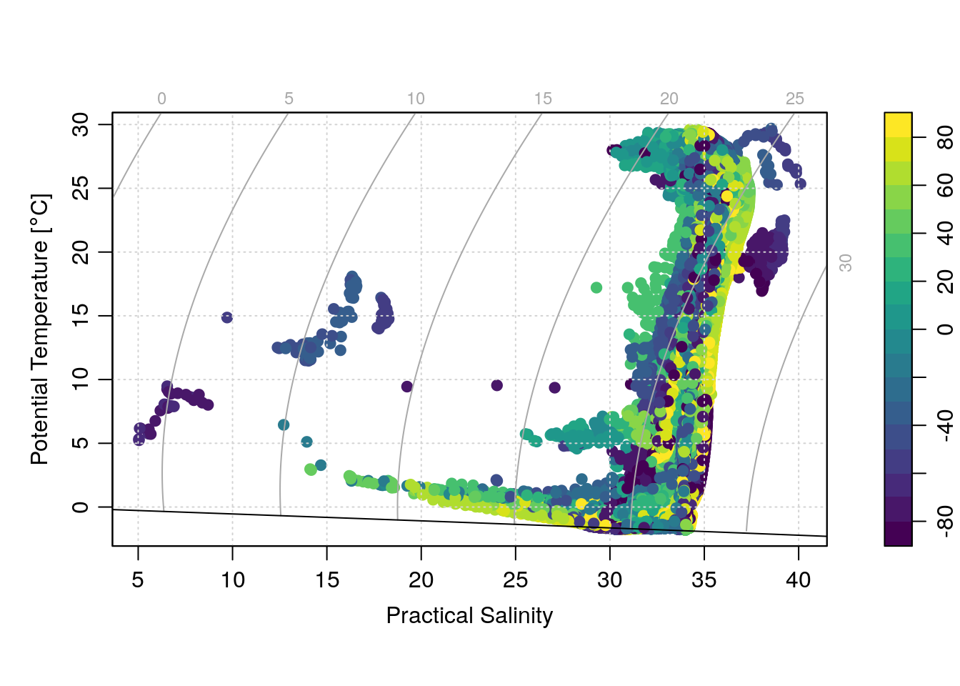
Custom color palettes with colormap()
In addition to the “known” color palettes that are included in R and oce (see also the cmocean package below, as well as RcolorBrewer), the colormap() function has arguments that allow for custom-built palettes. Specifically the x0, x1, col0 and col1 arguments, which are detailed in the help file as:
x0, x1, col0, col1: Vectors that specify a color map.  They must all be
          the same length, with ‘x0’ and ‘x1’ being numerical values,
          and ‘col0’ and ‘col1’ being colors.  The colors may be
          strings (e.g. ‘"red"’) or colors as defined by rgb or
          hsv.
The idea is that the x0 values define the numeric level of the bottom of the color ranges, the x1 values define the top of the color ranges, and the col0 and col1 the colors associated with the levels. An example:
cm <- colormap(expand.grid(levitus$latitude, levitus$longitude)[,1],
               x0=c(-90, -45, 0, 45), x1=c(-45, 0, 45, 90),
               col0=c(1, 2, 3, 4), col1=c(2, 3, 4, 5))
drawPalette(colormap=cm)
sI <- sample(seq_along(cm$zcol))
plotTS(with(levitus, as.ctd(SSS[sI], SST[sI], 0)), pch=19, col=cm$zcol[sI], mar=par('mar'))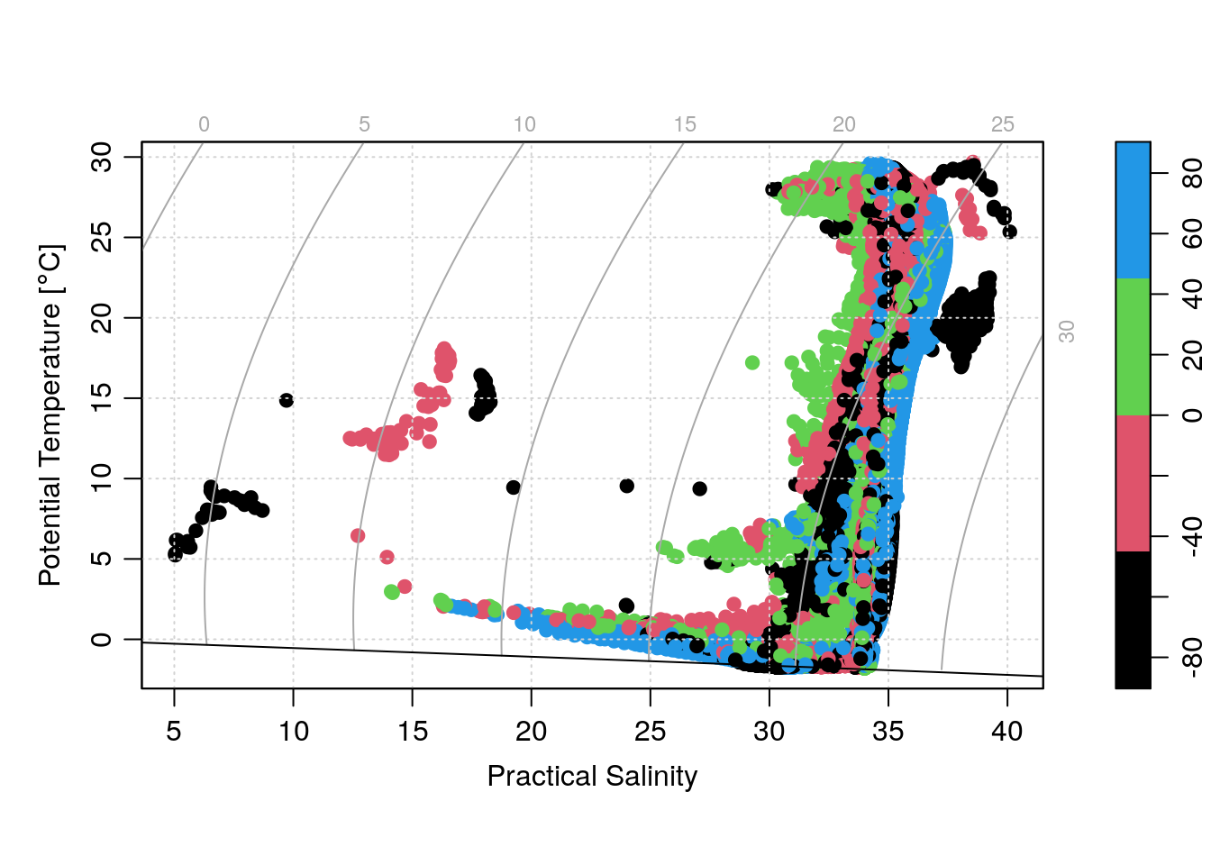
(Note that to make the above plot, I had to fix a bug in oce that was making the zcol come out as “black” for all cases. Either build oce from source, or wait for the update to get pushed to CRAN in a month or two).