
I love the \(\tanh\) function. A lot. It’s such a perfect model for a density interface in the ocean, that it is commonly used in theoretical and numerical models and I regularly used it for both research and demonstration/example purposes. Behold, a \(\tanh\) interface:
\[ T(z) = T_0 + \delta T \tanh \left( \frac{z-z_0}{dz} \right) \]
T <- function(z, T0=10, dT=5, z0=-25, dz=5) T0 + dT*tanh((z - z0)/dz)
z <- seq(0, -60)
plot(T(z), z)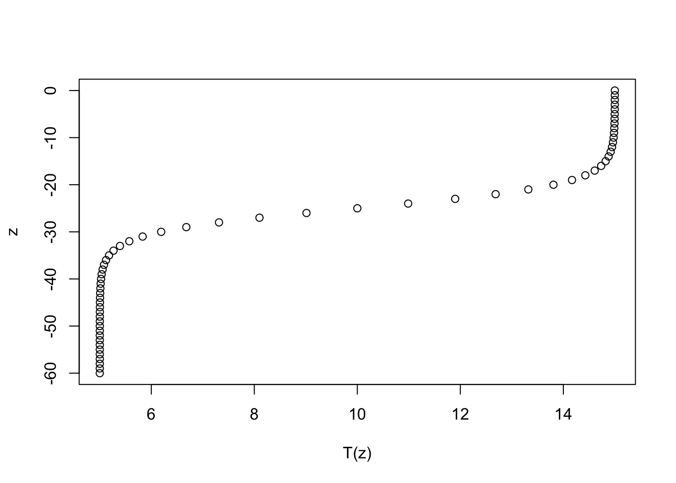
But whenever I use it, especially for teaching, I’m always saying how it’s idealized and really doesn’t represent what an ocean interface actually looks like. UNTIL NOW.
library(oce)
ctd <- read.oce('D19002034.ODF')
## Warning in read.odf(file = file, columns = columns, exclude = exclude, debug =
## debug - : "CRAT_01" should be unitless, but the file states the unit as "S/m" so
## that is retained in the object metadata. This will likely cause problems. See ?
## read.odf for an example of rectifying this unit error.par(mfrow=c(1, 2))
plot(ctd, which=1, type='l')
plot(ctd, which=5)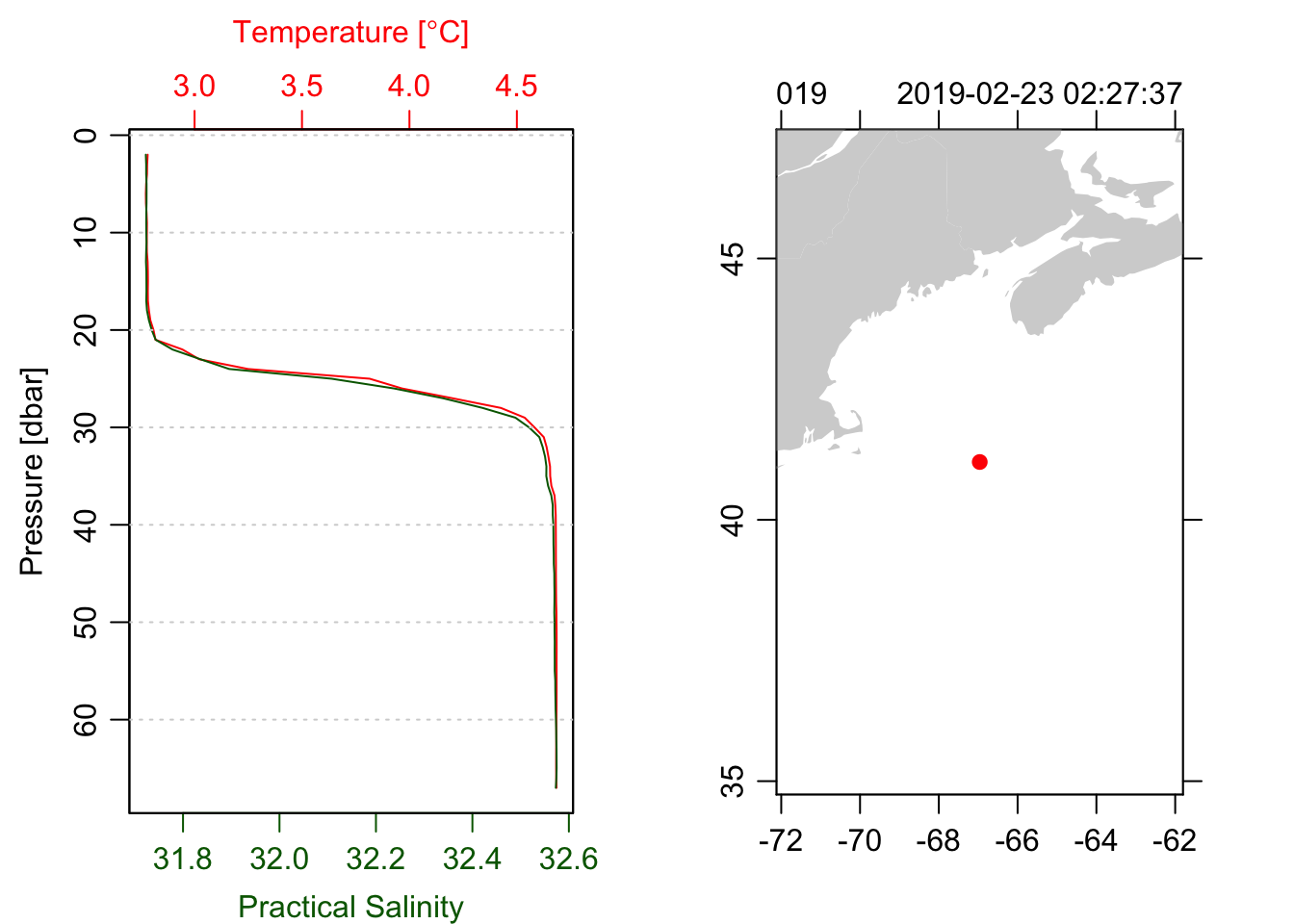
Yes, this is real data.
Just how close to a \(\tanh\) is it?1
z <- -ctd[["depth"]]
T <- ctd[["temperature"]]
m <- nls(T~a+b*tanh((z-z0)/dz), start=list(a=3, b=1, z0=-10, dz=5))
m
## Nonlinear regression model
## model: T ~ a + b * tanh((z - z0)/dz)
## data: parent.frame()
## a b z0 dz
## 3.7251 0.9516 -25.0448 -2.7648
## residual sum-of-squares: 0.05222
##
## Number of iterations to convergence: 16
## Achieved convergence tolerance: 4.394e-06plot((T-predict(m))/T * 100, z, type="o", xlab='Percent error')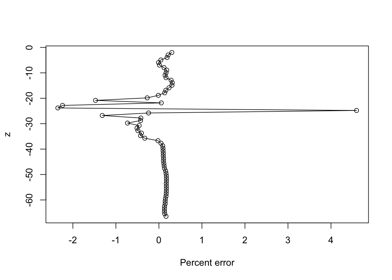
My PhD advisor, who also taught me introductory physical oceanography, once said to a class of students while using tanh to describe an idealized interface: “tanh – it’s like ‘lunch’, only better!”↩︎